Muzzle Velocity Stats – Statistics for Shooters Part 2

Consistent muzzle velocity is key for long-range shooting, otherwise, bullets that leave the muzzle faster than normal could miss high, or bullets that leave the muzzle slower could miss low. While the goal is for each shot to leave the muzzle at precisely the same velocity, no ammo is perfect. So it is very helpful for us as long-range shooters to understand the variation we can expect from our ammo shot-to-shot.

To see how much consistent muzzle velocity matters in terms of hit probability at long-range, read How Much Does SD Matter?

A primary goal of many long-range handloaders is to develop ammo with optimal muzzle velocity consistency, so this article will be 100% focused on helping us get more insight and make better decisions related to that. It will explain the different methods shooters use to quantify variation in velocity, dispel a few common misconceptions, and provide some practical tips.

Part 1 laid the foundation that we’ll build on here, so if you haven’t read it I’d start there. The next article, Part 3, will focus on the application of similar concepts when it comes to analyzing group size and dispersion.

Extreme Spread (ES) vs. Standard Deviation (SD)

The two most common stats shooters use to quantify variation in muzzle velocity are:

• Extreme Spread (ES): The difference between the slowest and fastest velocities recorded.
• Standard Deviation (SD): A measure of how spread out a set of numbers are. A low SD indicates all our velocities are closer to the average, while a high SD indicates the velocities are spread out over a wider range. (Note: Part 1 explained SD in detail, so please read that if you aren’t familiar with it – or the rest of this won’t make sense.)

Some shooters have strong opinions about which of those two measures are most applicable or relevant when it comes to long-range shooting, and they might completely ignore one or the other. But remember this important point from the last article, when it comes to any descriptive statistic, like ES or SD:

“Descriptive statistics [like ES and SD] are very good at summing up a bunch of data points into a single number. The bad news is that any simplification invites abuse. Descriptive statistics can be like online dating profiles: technically accurate and yet pretty darn misleading! Descriptive statistics exist to simplify, which always implies some loss of detail or nuance. So here is a very important point: An over-reliance on any descriptive statistic can lead to misleading conclusions.” – Charles Wheelan

So it’s probably a bad idea to be completely dismissive of either ES or SD. Both provide some form of insight. There are scenarios where SD is the best to use, and other scenarios where ES may be more helpful. I’ll try to provide a balanced perspective on when we should use one or the other.

In general, SD is usually a more reliable stat when it comes to quantifying the muzzle velocity variation. Adam MacDonald explains an important aspect when it comes to ES: “For normally distributed sample data, the extreme spread is a misleading measure of the variation because it ignores the bulk of the data and focuses entirely on whether extreme events happened to occur in that sample.” (Not sure what “normally distributed” means? Read Part 1.)

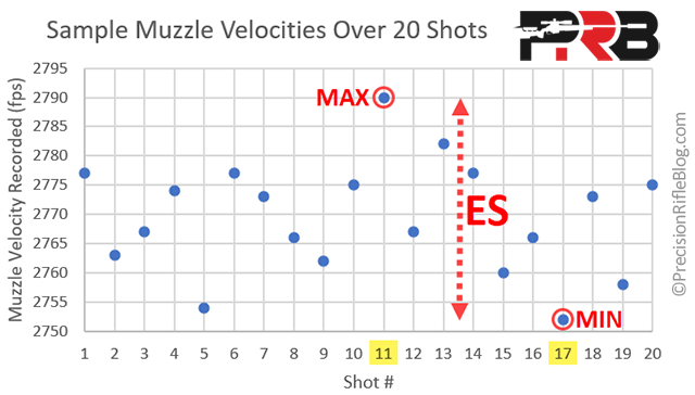
The example below shows muzzle velocities recorded over 20 shots, and we can see the ES is entirely dependent on the difference between shot #11 (the fastest) and #17 (the slowest). All of the other 18 shots are ignored when calculating ES. The ES is simply the max (2790 fps) minus the min (2752 fps): 2790 – 2752 = 38 fps.

The ES is by definition focused on the two most extreme values. MacDonald suggests, “We should instead be focusing on describing the results that are most likely to happen again. We need a metric which best represents the variation that we care about describing, and takes all the data into account. This is the standard deviation (SD).” He adds another important nuance between SD and ES: “As you collect more and more data, the measured SD of that sample becomes closer and closer to the true SD of the population. In contrast, the extreme spread will always grow with sample size, as more and more extreme events occur over time. It’s easier to measure, but it’s not nearly as reliable as the SD.”

MacDonald is not alone in this view. Most people who are familiar with statistics believe SD is a better statistical indicator of muzzle velocity variation. In fact, Engleman says it this plainly: “ES is not a reliable statistical indicator. The best indicator of velocity variations is the standard deviation.”

If we look back to the example of 20 muzzle velocities shown above, we can see how the ES grows as we fire more and more shots. The chart below shows what the ES was after each of the 20 shots. After the 2^nd shot, the max velocity is Shot #1 at 2777 fps and the min velocity is Shot #2 at 2763 fps, so our ES is 14 fps (2777 – 2763). Shots 3 and 4 land between those extremes, so the ES remains the same until Shot #5 registered down at 2754. That is 9 fps lower than our previous minimum, so at that point, our ES jumps up to 23 fps. Then it remains there until Shot #11 at 2790, which is 13 fps faster than our previous max of 2777, so our ES increases to 36 fps. Finally, Shot #17 registers at 2752, which is 2 fps slower than our previous minimum, so our ES grows to 38 fps. The chart below shows the progression of how ES changes over those 20 shots:

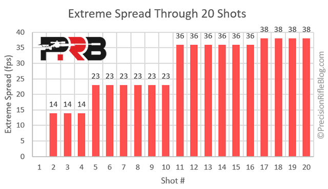
We can see if we’d have only fired 10 shots, we’d leave the range fully convinced that our ammo had an ES of 23 fps. But, when we fired shot #11, that one shot caused the ES to increase by over 50%! It was blind luck that round was Shot #11 and not Shot #2 or #20.

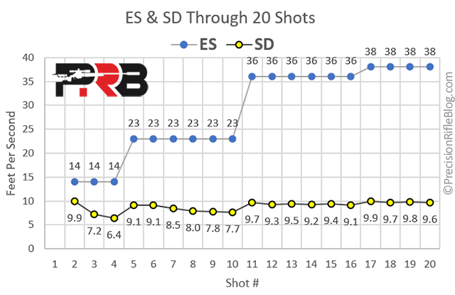
Because ES is ultimately based on two shots, a single shot could increase the ES drastically. However, because the SD is calculated using every data point, the more shots we fire, the less impact any single shot will have on the result. The chart below allows us to see how the SD starts to “stabilize” as the number of shots grows. The more shots fired, the less drastic the SD changes. However, the ES changes more sporadically through the 20 shots and would continue to increase if we continued to fire shots. If we fired 5 more shots, our ES might stay at 38 or go to 50+. However, it’s unlikely our SD would change drastically from what is shown. In fact, based on the 20-shot data we can predict with 90% confidence that even if we fired another 1,000 shots our SD would end up between 7.6 and 13.2 fps.

Some shooters believe ES is more applicable because they like to calculate if their shots would still hit a certain size target at their extreme fastest and slowest velocities. If their lowest muzzle velocity they recorded was 2,752 fps and their fastest was 2,790 fps, they could plug each of those into their ballistic calculator and see if the predicted drop would still result in an impact on a coyote-sized target at 600 yards. That seems relevant, right? But, if we have an accurate SD, we can actually use that to make a very good prediction of the true ES – possibly even more indicative of what the population might be than what we measured directly from a sample.

“The true extreme spread of a population is about 6 times the standard deviation,” explains Engleman. That is thanks to the power of a normal distribution, which we talked about in the last article. In a normal distribution, we know 99.9% of our shots will be within 3 SD (3 times the SD) from our average velocity. That means our slowest shot would be 3 times our SD below the average, and the fastest shot would be 3 times our SD above the average – and the difference between the min and the max would be very close to 6 times our SD. So, in our example where our SD is 9.6 fps, we should expect our ES to eventually grow to 58 fps if we continued to fire shots (9.6 fps SD x 6 = 57.6 fps ES). How many shots would it take before measured ES got to 58 fps? Who knows! It might take 100+ rounds, but we also might luck into that spread in a different 20-shot string. But, by 1,000 shots our data would take the shape of a normal distribution and our ES would likely land near 60 fps, yet our SD would very likely remain between 8 and 13 fps. This illustrates why SD is a more reliable statistical indicator of variation.

Is SD perfect? No! Any time we summarize a bunch of data with a single number, we are losing some nuance or detail. But, SD is certainly useful for quantifying muzzle velocity variation. Of course, there are some scenarios when ES might be more helpful, and I’ll try to point those out in this article.

What Is A “Good” SD?

If you’re newer to the concept of SD, you might be wondering, “What is a ‘good’ SD when it comes to muzzle velocity?”

It’s relatively easy for a reloader to produce ammo with an SD of 15 fps, but we typically have to be meticulous and use good components and equipment to wrestle that down into single digits. The table below is from Modern Advancements in Long Range Shooting Volume 2 and it provides a “summary of what kind of SD’s are required to achieve certain long-range shooting goals in general terms”:

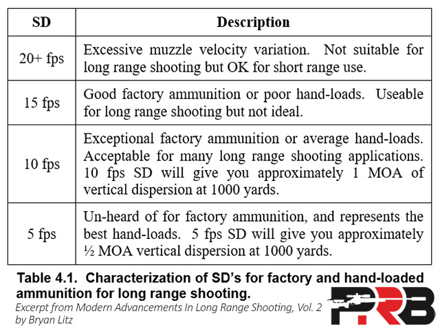
In general, most long-range shooters have a goal to have ammo with SD’s “in the single digits” (i.e. under 10 fps). Those engaging targets beyond 2,000 yards in Extreme Long Range (ELR), where first-round hits are critical, want to be closer to that 5 fps. The lower the better! 😉

For more context, read How Much Does SD Matter?

The Problem With SD: Sample Size Matters – A Lot!

At this point, we’ve established that SD is a superior statistical indicator of muzzle velocity variation, but there is a pitfall when it comes to SD that most shooters aren’t aware of: While it’s easy to get close to the average muzzle velocity with a smaller sample size, “but the SD is a different story. It’s a lot more difficult to measure variation than most people would assume,” explains MacDonald. If we want to have much confidence that our results represent the population we likely need a larger sample size than you think. Denton Bramwell agrees by saying, “Standard deviation is hard to estimate with precision.” Bramwell goes on to say that “changes in standard deviation are devilishly difficult to reliably detect,” and there is a “tendency to underestimate variation [and therefore SD] in small samples.” Engleman corroborates that point, saying, “Testing for velocity variations requires larger sample sizes – 5 shot samples will not yield reliable results.”

Many shooters see SD as an indicator of ammo quality (i.e. the lower the SD the higher the quality), so it’s common to see people brag about their low SD on the internet. They may even post a photo showing the stats from their LabRadar or MagnetoSpeed – and you can see it was over a 5 shot string. 5 shots is simply not a large enough sample size to have confidence in an SD. In fact, let’s say that someone had a 9 fps SD over 5 shots. For a 95% confidence interval, we would predict the real SD over a large sample size would be between 5.4 and 25.9 fps! The truth is, we can’t have much confidence in knowing our SD without a larger sample size. Many people record 10-shot strings, but the more the better! If we’re just trying to determine the average velocity, a 10-shot string is likely adequate, but when trying to quantify variation within a batch of ammo, we may need to record a string of 20 shots or more.

Engleman conducted a very interesting study where he recorded velocities over 50 consecutive shots, and then went back and grouped those results into distinct 5, 10, and 20 shot strings. He explained, “We will investigate scientifically sound methods of using 5, 10, or 20 shot strings to characterize a load combination. To do this, artificial strings will be chosen from the 50 shots already fired.” For example, forty-five 5 shot strings can be produced as follows:

• String 1: Shots # 1, 2, 3, 4, 5
• String 2: Shots # 2, 3, 4, 5, 6
• …
• String 45: Shots # 46, 47, 48, 49, 50

Note that we aren’t changing the order in which any shots were fired. Each of the strings includes shots captured in exact sequential order. If we only fired 5 shots from among the 50 recorded, it could have easily been any one of these artificial sets of sequential shots. Engleman followed the same method to create forty 10-shot strings and thirty 20-shot strings from the 50 sequential shots recorded.

His results show how much the average, SD, and ES could have varied based on the luck of the draw in terms of what shots happened to be included in each string:

Here is an important thing to notice: Think about if we are doing load development, and we’re trying to decide between two loads based on the SD of a 5-shot string we fired of each. This example shows that if we only fire a 5-shot string there is a chance we might measure an SD of 5 fps or 14 fps from the exact same batch of ammo! We’d obviously pick the load that produced the lower SD and might believe we had stumbled on a great load that is “tuned” for our rifle, although the lower SD was actually due to complete random chance and well within the natural variation we should expect from such a small sample size.

In Engleman’s results above, we can see the red lines change the most, which is the line indicating the possible output from a random set of 5 sequential shots. We can see on the top graph, depending on what 5 rounds we pulled out of the box, the average muzzle velocity might measure anywhere from 2982 fps to 2996 fps. Here is a summary of the ranges for each metric based on the number of shots in each group:

# of Shots In String	Average MV	SD	ES
5 Shots	2982-2996	4-14	12-40
10 Shots	2985-2992	7-12	20-40
20 Shots	2987-2989	8-11	30-45

Notice for all 3 metrics (average, SD, and ES), the more shots in each string the narrower the range of possible outcomes became. Simply put the more rounds we fire, the more certain we can be of the results. But, we can also see in the table above that as we fired more shots both the average and SD began to converge, but ES had a different pattern. The more rounds fired the higher the range of possible ES’s went. We shouldn’t be surprised that the highest ES occurred in the 20-shot string. That is part of the downside of ES: We should expect it to grow with sample size, where average and SD will begin to converge on the true value and don’t simply continue to grow the more shots we fire.

Here is Engleman’s key takeaway from his research:

“The first and most important fact presented in this paper is that random 5, 10, or 20 shot sequences all result in different statistics than the ones calculated for all 50 shots. In statistics, we refer to these smaller sequences as samples of the 50 shot population and the statistics generated by the samples are referred to as estimates of the population statistics. Thus, if during the winter off season I load 1000 rounds for competition, I may go to the range in the spring to estimate the expected performance of the total 1000 round population by randomly selecting 5, 10 or 20 rounds to test. I am not interested in the statistics of this sample shot sequence so much as we are interested in estimating the performance of the entire 1000 rounds. As can be seen from the data presented in Figure 3, it is very unlikely that the statistics from this sample will be exactly that of the 1000. To be clear, if you fire 5 shots from the 1000 you made over the winter over your chronograph and it tells you the SD = 4, then the standard deviation calculated for those 5 shots is exactly 4. But the standard deviation of all 1000 rounds is unlikely to be 4. The number presented on the chronograph is just an estimate of the total performance and the chronograph will not tell you how good a ‘guess’ it is.”

For SD in particular, Engleman went further and calculated the “90% Confidence Intervals” based on the number of shots in each string, and charted those along with the output for his “hypothetical strings” (if you aren’t sure what “confidence intervals” are, read Part 1):

We can see the range is the largest for the SD that is based on just 5 shots, and the range is much more narrow for the SD based on 10 shots and even tighter for the SD based on 20 shots. Engleman points out, “It is interesting to note that Sample #16 from the 5 shot samples is actually below the bound. 90% confidence means 1 in 10 chances may fail. String #16 was a very lucky string, but it was the only one of 45 possible strings outside the bounds which is much better than 90% success rate. Want better than 90% certainty? Either we have to make the confidence intervals wider or use more shots in the sample. There is no free lunch here – estimating standard deviations from samples is hard work.”

So, what is a good sample size? The answer depends on how minor the differences are that we’re trying to detect and how much confidence we want to have in the results being predictive of the future. When I am trying to quantify the variation in muzzle velocity for my ammo, I typically fire a minimum of 20 sequential shots. More recently, I’ve started taking my LabRadar with me when I practice long-range. Instead of only using it to record an occasional string of shots when I’m checking my zero or doing load development, I set it up and keep it running while I’m practicing from prone and I might record 30+ shots in a single range session. It doesn’t require me to fire any more rounds than I would have otherwise, but I’m simply gaining more value and insight about the true performance of my ammo.

During load development, we should also be cautious to draw conclusions from differences in SD’s that are a result of less than 20 shots. Even if we fired 10 shots of two different loads, and Load A had an SD of 8.3 fps and Load B had an SD of 11.5 fps – real statistics would tell us those are too close to know if one is truly superior to the other.

Bramwell explains, “As a rule of thumb, 22 data in each group is needed to detect a 1:2 ratio between two standard deviations, about 35 data in each group are required for a 2:3 ratio, and about 50 in each group are required for a 3:4 ratio. In a practical example, if you think you have lowered the standard deviation of your muzzle velocity from 20 to 15 fps, you’ll need to chronograph 100 rounds, 50 from each batch. If the ratio of the two standard deviations comes out 3:4 or greater, you’re justified in saying the change is real.”

As I mentioned in the last article, Adam MacDonald created an extremely helpful online calculator where we can enter our velocities for two loads and it will tell us how much confidence we can have that there is a true performance difference between the samples or if there is so much overlap it is more likely due to natural variation for the sample size we used. No crazy math or talk about F-Tests and P-Tests. Adam made it simple for us to input our data in plain English and get the results in plain English. Here is a link to Adam’s Stats Calculator for Shooters (alternate link).

It is very difficult to determine minor differences in variation between two loads without a ridiculously large sample size (like 100+ rounds each). Bramwell sums it up with this:

“Given the twin burdens of large sample size and sensitivity to non-normality, it is much more difficult than most people expect to tell if a change in standard deviation is real, or if it was just our lucky day.  Consequently, a lot of people perform tests, and draw conclusions on truly insufficient data.”

I’ve heard a respected researcher say he usually only pays attention to differences of 15% or more, and even when his team finds those, they’ll fire more rounds to confirm what they’re seeing is real and not simply random variation from a smaller sample size.

Correcting For Smaller Sample Sizes

I realize most of us aren’t going to fire 100 or even 30 round samples for each powder charge and seating depth we try in our load development. So is there something we can do to make better decisions when working with 3 to 10 shot groups?

When we have very small sample sizes, we must realize that variation is typically under-estimated. In fact, when a sample has less than 30 observations, statisticians often apply correction factors to adjust for that.

“When we measure the outcome of a random process just a few times, we tend to underestimate the true variation. That is, if we continue to measure the outcome, the standard deviation of the (increasing) sample size tends to increase. This is very important for shooters because we typically judge performance based on 3-10 shot groups,” explains Bruce Winker. “Range data must be corrected for this effect. … To get a more accurate estimate of the standard deviation of the actual distribution, we will need to apply a correction factor to the group size and muzzle velocity data that we measure at the range.” Bruce explains more about how that works in A User’s Guide To Dispersion Analysis.

Instead of applying a correction factor, Bramwell suggests another approach: “For samples as small as five or so, use range [e.g. ES] instead of standard deviation.” Very small sample sizes are one of those niche scenarios where ES can be a useful stat.

ES can help us eliminate or rule-out loads early on. This is based on the principle that over the long haul we can expect our ES to be around 6 times our SD, right? So, if our measured ES is more than 6 times whatever our SD goal is, we know that load isn’t going to get us there.

Adam MacDonald agrees with Bramwell, sharing his rule of thumb: “Use extreme spread to rule out a bad load with 5 shots. Use standard deviation to prove a good load with confidence.”

Let’s say we are developing a load for Extreme Long Range competitions and our goal is to find a load that produces an SD around 7 fps or less. If our goal for SD is 7 fps, then we expect our ES will be 42 fps (7 x 6 = 42). If after a few shots with a certain load our ES is already 50 fps or more, it’s a safe bet that load isn’t going to get us there and we can move on. Because we expect ES to grow as our sample size grows, we’d likely want to see an ES closer to 4 times the SD over smaller sample sizes (7 x 4 = 28 fps).

How Good Is Your Chronograph?

The final tip I’ll mention about quantifying the variation in muzzle velocity is to understand how precise your chronograph is. Most cheap, light-based chronographs aren’t very precise, and they will add “noise” to your data. If we’re trying to measure SD’s for our ammo into single digits, but our chronograph has 10 fps of SD in its readings – we have a problem! Bryan Litz did a very helpful test of consumer-grade chronographs several years ago, and his results were published in detail in Modern Advancements for Long Range Shooting Volume 1, and I noticed AB also published the full chapter featuring this test online. The chart below shows a summary of the amount of error Bryan measured:

We can see the Oehler 35P produced the most impressive results, with an SD around 1 fps in the equipment readings. The popular MagnetoSpeed had an SD of 3-4 fps. The Shooting Chrony (discontinued) had an SD around 3 fps, but the average it reported was off by 18-22 fps – so I’d call that precise (repeatable), but not accurate (far from the correct value). Beyond those, it quickly turns into a mess. The PVM-21 and SuperChrono were just disasters, in terms of precision and accuracy.

The very popular LabRadar Doppler Radar was released after the Applied Ballistics team did this test. While many people are big fans of the LabRadar, I’m unaware of an objective, third-party test that has been done with the same level of rigor as the Applied Ballistics study. The manufacturer does claim the “LabRadar has an accuracy of 0.1%.” For a reading of 3,000 fps that would be an accuracy of +/- 3 fps, which seems to be comparable with the better chronographs in the Applied Ballistics tests. The anecdotal comparisons (like this one published on AccurateShooter.com, or this comparison against a professional Weibel Doppler Radar) appear to indicate it has similar accuracy and precision to the Oehler 35P and MagnetoSpeed.

If there is noise being added by the measurement device, one way proven way to separate the signal from the noise is to increase the sample size. No surprise at this point! If we want more confidence in the data, the proven path is to simply collect more of it!

Summary & Key Points

We covered a lot of ground, so let’s review some of the key points from this article:

• It’s probably a bad idea to be completely dismissive of either ES or SD. Both provide some form of insight. An over-reliance on any descriptive statistic can lead to misleading conclusions.
• SD is a more reliable and effective stat when it comes to quantifying muzzle velocity variations. ES is easier to measure but is a weaker statistical indicator in general because it is entirely based on the two most extreme events.
• ES will grow with sample size, but average and SD will begin to converge on the true value and don’t simply continue to grow the more shots we fire.
• While it’s easy to get close to the average muzzle velocity with 10 shots or less, it’s exceedingly more difficult to measure variation and SD with precision. There is a tendency for SD to be understated in small samples. To have much confidence that our SD is accurate, we need a larger sample size than many would think – likely 20-30 shots or more. The more the better!
• It is very difficult to determine minor differences in velocity variation between two loads without a ridiculously large sample size (like 50+ rounds or more of each load to differentiate even a 20% difference). Often we make decisions based on truly insufficient data because the measured performance difference between two loads is simply a result of the natural variation we can expect in small sample sizes.
• ES can help to eliminate bad loads early but use SD to prove a good load with confidence.

Other Articles In This Series

Stay tuned for the final article in this series, where we’ll turn our focus to group size and how we can get the most out of the groups we fire and leverage those to make more informed decisions and get more rounds on target.

1. How To Predict The Future: Fundamentals of statistics for shooters
2. Quantifying Muzzle Velocity Consistency: Gaining insight to minimize our shot-to-shot variation in velocity (this article)
3. Quantifying Group Dispersion: Making better decisions when it comes to precision and how small our groups are
4. Executive Summary: This article recaps the key points from all 3 articles in a brief bullet-point list

You can also view my full list of works cited if you’re interested in diving deeper into any of these topics.